Neighborhood Analysis: GIS
Neighborhood analysis evaluates the spatial relationship between a cell and its neighboring cells (in raster data) or a feature and its nearby features (in vector data).
Introduction
The GIS filtering process is sometimes referred to as scanning but is not to be confused with data capture via a digital camera. Neighborhood analysis is based on local or neighborhood characteristics of the data (Star and Estes, 1990).
Every pixel is analyzed spatially, according to the pixels that surround it. The number and the location of the surrounding pixels is determined by a scanning window, which is defined by you.
These operations are known as focal operations. The scanning window can be of any size in SML. In Model Maker, it has the following constraints:
- Circular, with a maximum diameter of 512 pixels
- Doughnut-shaped, with a maximum outer radius of 256
- Rectangular, up to 512 × 512 pixels, with the option to mask-out certain
- pixels
Defining Scan Area
You may define the area of the file to be scanned. The scanning window moves only through this area as the analysis is performed. Define the area in one or all of the following ways:
- Specify a rectangular portion of the file to scan. The output layer contains only the specified area.
- Specify an area that is defined by an existing AOI layer, an annotation overlay, or a vector layer. The area or areas within the polygon are scanned, and the other areas remain the same. The output layer is the same size as the input layer or the selected rectangular portion.
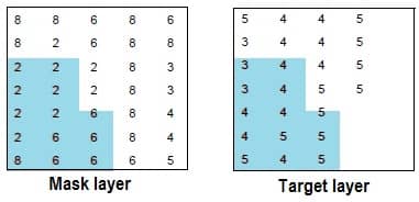
- Specify a class or classes in another thematic layer to be used as a mask. The pixels in the scanned layer that correspond to the pixels of the selected class or classes in the mask layer are scanned, while the other pixels remain the same.
Create Thematic Layer with Neighborhood Analysis
Neighborhood analysis creates a new thematic layer. There are several types of analysis that can be performed upon each window of pixels, as described below:
- Boundary—detects boundaries between classes. The output layer contains only boundary pixels. This is useful for creating boundary or edge lines from classes, such as a land/water interface.
- Density—outputs the number of pixels that have the same class value as the center pixel. This is also a measure of homogeneity, based upon the analyzed pixel. This is often useful in assessing vegetation crown closure.
- Diversity—outputs the number of class values that are present within the window. Diversity is also a measure of heterogeneity.
- Majority—outputs the class value that represents the majority of the class values in the window. The value is defined by you. This option operates like a low-frequency filter to clean up a salt and pepper layer.
- Maximum—outputs the greatest class value within the window. This can be used to emphasize classes with the higher class values or to eliminate linear features or boundaries.
- Mean—averages the class values. If class values represent quantitative data, then this option can work like a convolution filter. This is mostly used on ordinal or interval data.
- Median—outputs the statistical median of the class values in the window. This option may be useful if class values represent quantitative data.
- Minimum—outputs the least or smallest class value within the window. The value is defined by you. This can be used to emphasize classes with the low class values.
- Minority—outputs the least common of the class values that are within the window. This option can be used to identify the least common classes. It can also be used to highlight disconnected linear features.
- Rank—outputs the number of pixels in the scan window whose value is less than the center pixel.
- Standard deviation—outputs the standard deviation of class values in the window.
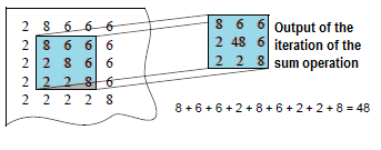
- Sum—totals the class values. In a file where class values are ranked, use totaling to further rank pixels based on their proximity to high-ranking pixels.
Neighborhood Analysis in GIS
In GIS Neighborhood Analysis refers to analyzing the characteristics of surrounding features or cells in relation to a focal location. It is widely used in raster analysis, particularly in environmental modeling, urban planning, and landscape analysis.
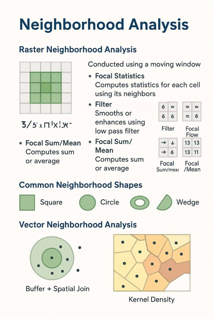
Raster Neighborhood Analysis
This is the most common form and is conducted using a moving window (typically 3×3, 5×5, etc.).
🔧 Tools in ArcGIS Pro (Spatial Analyst Toolbox → Neighborhood):
| Tool | Description |
|---|---|
| Focal Statistics | Computes statistics (mean, max, std dev, etc.) for each cell using its neighbors. |
| Filter | Smooths or enhances a raster image using low-pass (mean) or high-pass (edge) filters. |
| Focal Flow | Determines flow direction based on slope between a cell and its neighbors. |
| Focal Sum/Mean | Computes the sum or average of surrounding cell values. |
Common Neighborhood Shapes:
- Square (3×3, 5×5)
- Circle
- Annulus (ring-shaped)
- Wedge
Vector Neighborhood Analysis
Involves finding features within a specified distance or criteria.
Tools:
- Buffer + Spatial Join (to count or summarize nearby features)
- Near (adds distance to nearest feature)
- Point Density / Kernel Density
Example: Find how many schools are within 1 km of each hospital.
Applications
- Heatmap generation (Kernel Density)
- Slope and aspect analysis (terrain)
- Urban heat island mapping
- Habitat suitability modeling
- Site selection